Homework 1

Assigned: Apr 9, 2021
Due: Apr 23, 2021
Assignments Homework

Background

There are three primary purposes for this homework:

Practice restructuring data in a format that would be appropriate for multilevel modeling in R via the {lme4} package
Fitting models you are already familiar with through R, rather than through HLM or other proprietary software.
Creating a few basic plots of the model results

Getting started

Create a new RStudio project for this homework. Create a folder for the data and place “longitudinal-sim.csv” in that folder. Create a new R markdown file to complete the lab. You can use whatever basic format you’d like, but please make it clear which question you are addressing, in each code chunk, keep text outside of code chunks (unless there are specific parts of the code you’d like to comment), and avoid printing large output. In other words, you can do whatever exploratory work you need to do, but please remove (or comment out) any code that ends up printing anything that is not directly related to your response (e.g., a data frame).

Part 1: Data structuring

Read in the “longitudinal-sim.csv” file. It should look like the below.

## # A tibble: 22,500 x 12
##    distid scid  sid     g3_fall g3_winter g3_spring  g4_fall g4_winter g4_spring
##     <dbl> <chr> <chr>     <dbl>     <dbl>     <dbl>    <dbl>     <dbl>     <dbl>
##  1      1 1-1   1-1-1  203.0107  202.4761  212.2639 205.3442  214.2586  220.2867
##  2      1 1-1   1-1-2  195.4607  197.2084  198.3835 202.8677  202.5952  214.1419
##  3      1 1-1   1-1-3  176.7393  186.8664  194.8692 188.0653  195.2954  203.0824
##  4      1 1-1   1-1-4  177.4862  189.6411  185.9529 184.8689  184.6891  201.9689
##  5      1 1-1   1-1-5  177.8235  191.6727  190.3565 194.1273  197.9155  201.9845
##  6      1 1-1   1-1-6  199.6338  200.5751  212.9278 200.3407  215.8191  230.8688
##  7      1 1-1   1-1-7  191.6022  192.1096  209.7669 204.0859  207.3352  215.3286
##  8      1 1-1   1-1-8  178.1014  200.9007  198.3188 202.6612  209.3969  213.9135
##  9      1 1-1   1-1-9  195.4754  191.6468  203.9326 195.2835  207.3704  206.8144
## 10      1 1-1   1-1-10 213.4238  207.6226  215.9710 207.8315  214.3541  232.6554
## # … with 22,490 more rows, and 3 more variables: g5_fall <dbl>,
## #   g5_winter <dbl>, g5_spring <dbl>

Each row in this dataset represents a student (sid) nested in a school (scid) nested in a school district (distid). The remaining columns represent scores from a seasonally-administered benchmark assessment (administered in the fall, winter, and spring) across Grades 3-5.

Restructure this dataset so you could use the {lme4} package to fit a growth model with random intercepts and slopes for students and grade-level fixed effects. Code time by wave (e.g., fall, winter, spring = 0, 1, 2).

Note: Depending on your comfort level with R, this may be quite challenging. Please make sure to work with your group members and/or check in with me. The important part is that you understand how to do this, not neccessarily that you complete it this one time. There are also lots of different ways to do this, so don’t get too hung up on one “correct” way.

Part 2: Model fit and evaluation

Part A

Fit the following models with student-level random effects (i.e., ignoring any potential school- or district-level variability for now):

Unconditional growth model with random intercepts and parallel slopes
Conditional growth model with random intercepts, parallel slopes, and grade-level fixed effects
Unconditional growth model with random intercepts and random slopes
Conditional growth model with random intercepts, random slopes, and grade-level fixed effects

Note when I ran models 3 and 4 I did run into some convergence warnings. You can safely ignore these, or you can use a different optimizer to get rid of them by adding control = lmerControl(optimizer = "bobyqa"). The {lme4} package has several possible optimizer and, in this case, the default optimizer did not quite reach its tolerance for convergence, while most of the others do.

Part B

Compare the performance of the four models you fit in the previous section. Which model displays the best fit to the data? Make a determination and provide a brief writup, using evidence to justify your selection.

Part C

Provide a brief writeup interpreting the model you selected from above. Be sure to interpret both the fixed effects and random effects. I’m looking for a “plain English” description. It does not necessarily need to be APA style, but plain English and APA are also not mutually exclusive, so you could. Please make sure to also include confidence intervals in your interpretation.

Part 3: Plots of the model fit

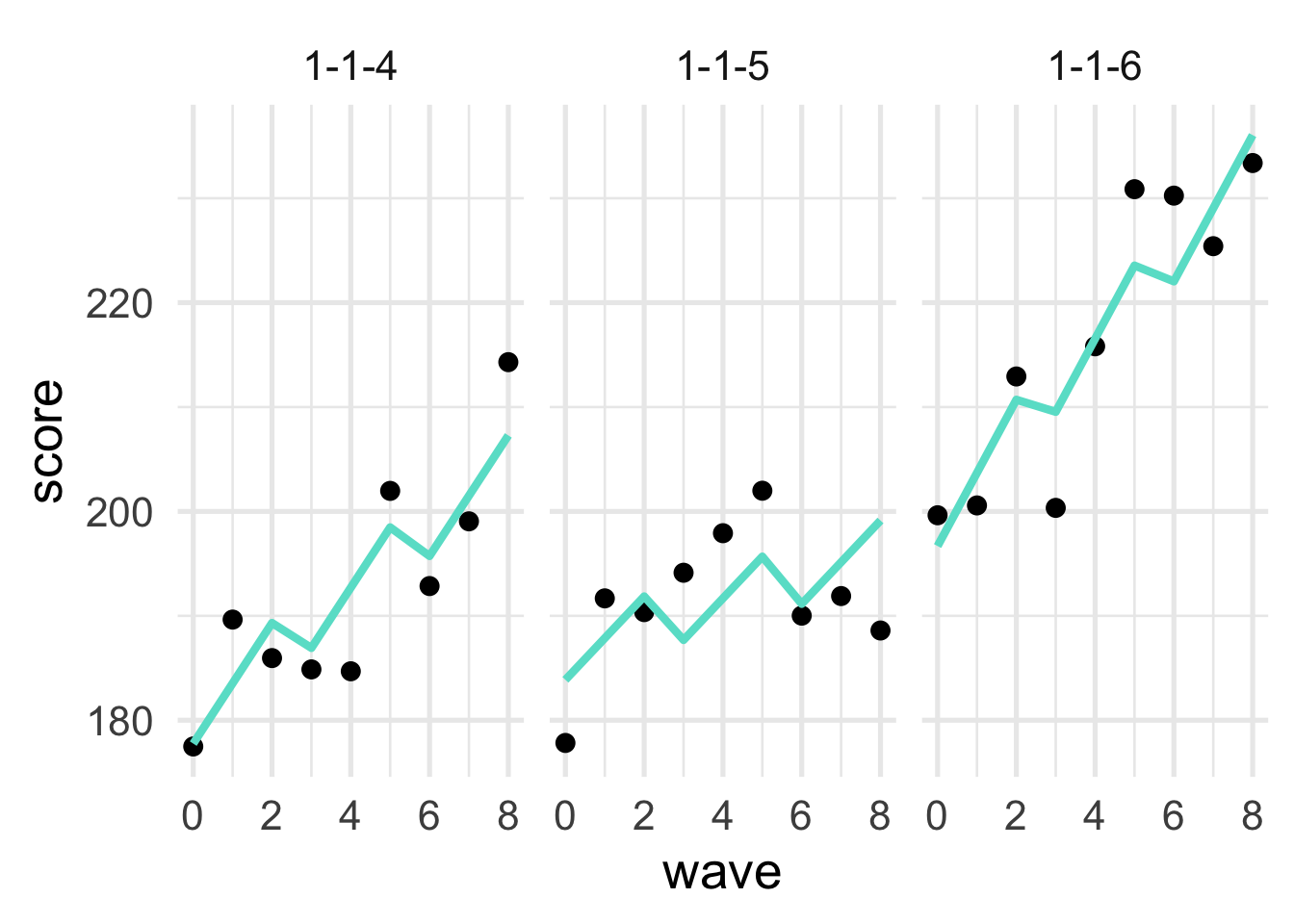
Plot the predicted values for student ID’s 1-1-1, 1-1-2, and 1-1-3, relative to their observed data points. Use facet wrapping to place them all in the same plot. The end result should look similar to the below, which shows this relation for student IDS 1-1-4, 1-1-5, and 1-1-6. Note that my plot has some styling added to it which you can feel free to ignore (I just can’t help myself).