Agenda

• Fitting some basic models

• Coefficient plots

• Using the coefficients to make predictions "by hand"

  • contrast with results from predict()

• Building predictions for new data

• Marginal effects

Learning objectives

• Understand how to pull different pieces out of the model

• Understand how multilevel models make their predictions for individual observations

  • And specifically how they differ from single-level regression models

• Be able to use the output from model objects to visualize different parts of the model.

Read in the data

Let's read in the popularity data so we can fit some really basic models.

You try first

library(tidyverse)
popular <- read_csv(here::here("data", "popularity.csv"))
popularCopy Code

## # A tibble: 2,000 x 7
##    pupil class extrav sex    texp popular popteach
##    <dbl> <dbl>  <dbl> <chr> <dbl>   <dbl>    <dbl>
##  1     1     1      5 girl     24     6.3        6
##  2     2     1      7 boy      24     4.9        5
##  3     3     1      4 girl     24     5.3        6
##  4     4     1      3 girl     24     4.7        5
##  5     5     1      5 girl     24     6          6
##  6     6     1      4 boy      24     4.7        5
##  7     7     1      5 boy      24     5.9        5
##  8     8     1      4 boy      24     4.2        5
##  9     9     1      5 boy      24     5.2        5
## 10    10     1      5 boy      24     3.9        3
## # … with 1,990 more rowsCopy Code

Fit a basic model

Fit each of the following models

• popular as the outcome, with a random intercept for class

• popular as the outcome, with sex included as a fixed effect and a random intercept for class

• popular as the outcome, with sex included as a fixed effect and a random intercept and slope for class

Models

library(lme4)
m0 <- lmer(popular ~ 1 + (1|class), popular)
m1 <- lmer(popular ~ sex + (1|class), popular)
m2 <- lmer(popular ~ sex + (sex|class), popular)Copy Code

Compare performance

Use whatever tests you'd like, and come up with the model you think fits the data best

library(performance)
compare_performance(m0, m1, m2) %>% 
  print_md()Copy Code

Table: Comparison of Model Performance Indices

Test of the Log-likelihood

test_likelihoodratio(m0, m1) %>% 
  print_md()Copy Code

test_likelihoodratio(m1, m2) %>% 
  print_md()Copy Code

Pretty good evidence that m1 displays the best fit

Package options

The {parameters} package (part of the {easystats} ecosystem) will get you where you want to be.

Alternatively, you could use the {broom.mixed} package (which is a spin-off of the {broom} package) which requires slightly less code.

I'll illustrate both

install.packages("broom.mixed")Copy Code

{broom.mixed}

library(broom.mixed)
tidy(m0)Copy Code

## # A tibble: 3 x 6
##   effect   group    term             estimate   std.error statistic
##   <chr>    <chr>    <chr>               <dbl>       <dbl>     <dbl>
## 1 fixed    <NA>     (Intercept)     5.077860   0.08739443  58.10278
## 2 ran_pars class    sd__(Intercept) 0.8379169 NA           NA      
## 3 ran_pars Residual sd__Observation 1.105348  NA           NACopy Code

Or get just the fixed effects

tidy(m0, effects = "fixed")Copy Code

## # A tibble: 1 x 5
##   effect term        estimate  std.error statistic
##   <chr>  <chr>          <dbl>      <dbl>     <dbl>
## 1 fixed  (Intercept) 5.077860 0.08739443  58.10278Copy Code

Across models

Let's tidy all three models, extracting just the fixed effects, and adding in a 95% confidence interval

models <- bind_rows(
  tidy(m0, effects = "fixed", conf.int = TRUE),
  tidy(m1, effects = "fixed", conf.int = TRUE),
  tidy(m2, effects = "fixed", conf.int = TRUE),
  .id = "model"
  ) %>% 
  mutate(model = as.numeric(model) - 1)
modelsCopy Code

## # A tibble: 5 x 8
##   model effect term        estimate  std.error statistic conf.low conf.high
##   <dbl> <chr>  <chr>          <dbl>      <dbl>     <dbl>    <dbl>     <dbl>
## 1     0 fixed  (Intercept) 5.077860 0.08739443  58.10278 4.906570  5.249150
## 2     1 fixed  (Intercept) 4.394460 0.07586494  57.92478 4.245767  4.543152
## 3     1 fixed  sexgirl     1.350102 0.04403301  30.66113 1.263799  1.436405
## 4     2 fixed  (Intercept) 4.396820 0.08012978  54.87123 4.239768  4.553871
## 5     2 fixed  sexgirl     1.352175 0.05029920  26.88263 1.253590  1.450760Copy Code

Plot

pd <- position_dodge(0.5)
ggplot(models, aes(estimate, term, color = factor(model))) +
  geom_errorbarh(aes(xmin = conf.low, xmax = conf.high), 
                 position = pd,
                 height = 0.2) +
  geom_point(position = pd)Copy Code

Standardization

The nice thing about tidying the model output, is that the code on the previous slides will always work regardless of the model(s) you've fit.

Caveat

I don't actually think the prior plot is all that useful.

• Occasionally helpful to visualize differences between coefficients, but you'll usually want to omit the intercept

• Be careful about scales

• If you were to publish the prior plot, make it prettier and more accessible first

{parameters}

To get basically the same output from parameters:

library(parameters)
parameters(m0) %>% 
  as_tibble()Copy Code

## # A tibble: 1 x 10
##   Parameter   Coefficient         SE    CI   CI_low  CI_high        t df_error
##   <chr>             <dbl>      <dbl> <dbl>    <dbl>    <dbl>    <dbl>    <int>
## 1 (Intercept)    5.077860 0.08739443  0.95 4.906570 5.249150 58.10278     1997
## # … with 2 more variables: p <dbl>, Effects <chr>Copy Code

models2 <- bind_rows(
  as_tibble(parameters(m0)),
  as_tibble(parameters(m1)),
  as_tibble(parameters(m2)),
  .id = "model"
  ) %>% 
  mutate(model = as.numeric(model) - 1)Copy Code

pd <- position_dodge(0.5)
ggplot(models2, aes(Coefficient, Parameter, 
                    color = factor(model))) +
  geom_errorbarh(aes(xmin = CI_low, xmax = CI_high), 
                 position = pd,
                 height = 0.2) +
  geom_point(position = pd)Copy Code

Other parts of the model

From here on out, I'll just be using {broom.mixed} but either package should work, with minor tweaks.

Variance components

Notice that, by default, we don't have any uncertainty

tidy(m0)Copy Code

## # A tibble: 3 x 6
##   effect   group    term             estimate   std.error statistic
##   <chr>    <chr>    <chr>               <dbl>       <dbl>     <dbl>
## 1 fixed    <NA>     (Intercept)     5.077860   0.08739443  58.10278
## 2 ran_pars class    sd__(Intercept) 0.8379169 NA           NA      
## 3 ran_pars Residual sd__Observation 1.105348  NA           NACopy Code

We can fix this by using bootstrap or profiled CIs

Bootstrap CIs

tidy(
  m0,
  effects = "ran_pars", 
  conf.int = TRUE, 
  conf.method = "boot"
)Copy Code

## Computing bootstrap confidence intervals ...Copy Code

## # A tibble: 2 x 6
##   effect   group    term             estimate  conf.low conf.high
##   <chr>    <chr>    <chr>               <dbl>     <dbl>     <dbl>
## 1 ran_pars class    sd__(Intercept) 0.8379169 0.7145176 0.9652536
## 2 ran_pars Residual sd__Observation 1.105348  1.071117  1.141232Copy Code

m2

Note this takes a bit of time, even though the model is pretty simple. Also these are standard deviations and a correlation, not variances/covariances

tidy(
  m2,
  effects = "ran_pars", 
  conf.int = TRUE, 
  conf.method = "boot"
)Copy Code

## Computing bootstrap confidence intervals ...Copy Code

## 
## 35 message(s): boundary (singular) fit: see ?isSingular
## 16 warning(s): Model failed to converge with max|grad| = 0.00213278 (tol = 0.002, component 1) (and others)Copy Code

## # A tibble: 4 x 6
##   effect   group    term                       estimate    conf.low  conf.high
##   <chr>    <chr>    <chr>                         <dbl>       <dbl>      <dbl>
## 1 ran_pars class    sd__(Intercept)           0.7389520  0.6133643  0.8469480 
## 2 ran_pars class    cor__(Intercept).sexgirl -0.4442543 -1          0.04996563
## 3 ran_pars class    sd__sexgirl               0.2336921  0.04570838 0.3513648 
## 4 ran_pars Residual sd__Observation           0.9049626  0.8744993  0.9341371Copy Code

Quick challenge

Can you make a dotplot with uncertainty for the variance components?

What about a plot showing both fixed effects and variance components?

One approach

pull_model_results <- function(model) {
  tidy(
    model,
    conf.int = TRUE, 
    conf.method = "boot"
  )
}
full_models <- bind_rows(
  pull_model_results(m0),
  pull_model_results(m1),
  pull_model_results(m2),
  .id = "model"
)Copy Code

## Computing bootstrap confidence intervals ...
## Computing bootstrap confidence intervals ...
## Computing bootstrap confidence intervals ...
## Computing bootstrap confidence intervals ...
## Computing bootstrap confidence intervals ...Copy Code

## 
## 30 message(s): boundary (singular) fit: see ?isSingular
## 13 warning(s): Model failed to converge with max|grad| = 0.00215039 (tol = 0.002, component 1) (and others)Copy Code

## Computing bootstrap confidence intervals ...Copy Code

## 
## 30 message(s): boundary (singular) fit: see ?isSingular
## 9 warning(s): Model failed to converge with max|grad| = 0.00203702 (tol = 0.002, component 1) (and others)Copy Code

ggplot(full_models, aes(estimate, term, color = factor(model))) +
  geom_errorbarh(aes(xmin = conf.low, xmax = conf.high), 
                 position = pd,
                 height = 0.2) +
  geom_point(position = pd) +
  facet_wrap(~effect, scales = "free_y") +
  theme(legend.position = "bottom")Copy Code

Random effects

Pop Quiz

What's the difference between the output from below and the output on the next slide?

tidy(m0, effects = "ran_vals")Copy Code

## # A tibble: 100 x 6
##    effect   group level term            estimate std.error
##    <chr>    <chr> <chr> <chr>              <dbl>     <dbl>
##  1 ran_vals class 1     (Intercept) -0.002630828 0.2370649
##  2 ran_vals class 2     (Intercept) -0.8949875   0.2370649
##  3 ran_vals class 3     (Intercept) -0.3496155   0.2487845
##  4 ran_vals class 4     (Intercept)  0.3318175   0.2222273
##  5 ran_vals class 5     (Intercept)  0.1919485   0.2317938
##  6 ran_vals class 6     (Intercept) -0.6833977   0.2370649
##  7 ran_vals class 7     (Intercept) -0.8062842   0.2317938
##  8 ran_vals class 8     (Intercept) -1.019181    0.2370649
##  9 ran_vals class 9     (Intercept) -0.3844123   0.2370649
## 10 ran_vals class 10    (Intercept)  0.2226622   0.2178678
## # … with 90 more rowsCopy Code

tidy(m0, effects = "ran_coefs")Copy Code

## # A tibble: 100 x 5
##    effect    group level term        estimate
##    <chr>     <chr> <chr> <chr>          <dbl>
##  1 ran_coefs class 1     (Intercept) 5.075229
##  2 ran_coefs class 2     (Intercept) 4.182872
##  3 ran_coefs class 3     (Intercept) 4.728244
##  4 ran_coefs class 4     (Intercept) 5.409677
##  5 ran_coefs class 5     (Intercept) 5.269808
##  6 ran_coefs class 6     (Intercept) 4.394462
##  7 ran_coefs class 7     (Intercept) 4.271575
##  8 ran_coefs class 8     (Intercept) 4.058678
##  9 ran_coefs class 9     (Intercept) 4.693447
## 10 ran_coefs class 10    (Intercept) 5.300522
## # … with 90 more rowsCopy Code

Answer

The output from ran_vals provides the estimate from ${\alpha }_j\sim N(0,\sigma )$.

The output from ran_coefs provides the class-level predictions, i.e., in this case, the intercept + the estimated ran_vals.

Example

tidy(m0, effects = "ran_vals")$estimate[1:5] + fixef(m0)[1]Copy Code

## [1] 5.075229 4.182872 4.728244 5.409677 5.269808Copy Code

tidy(m0, effects = "ran_coefs")$estimate[1:5]Copy Code

## [1] 5.075229 4.182872 4.728244 5.409677 5.269808Copy Code

Let's plot the ran_vals

m0_ranvals <- tidy(m0, effects = "ran_vals", conf.int = TRUE)
ggplot(m0_ranvals, aes(level, estimate)) +
  geom_errorbar(aes(ymin = conf.low, ymax = conf.high),
                width = 0.2) +
  geom_point() +
  geom_hline(yintercept = 0, size = 2, color = "magenta")Copy Code

Not super helpful

Try again

Let's reorder the level according to the estimate

m0_ranvals %>% 
  mutate(level = reorder(factor(level), estimate)) %>%
  ggplot(aes(level, estimate)) +
  geom_errorbar(aes(ymin = conf.low, ymax = conf.high),
                width = 0.5) +
  geom_point() +
  geom_hline(yintercept = 0, size = 2, color = "magenta")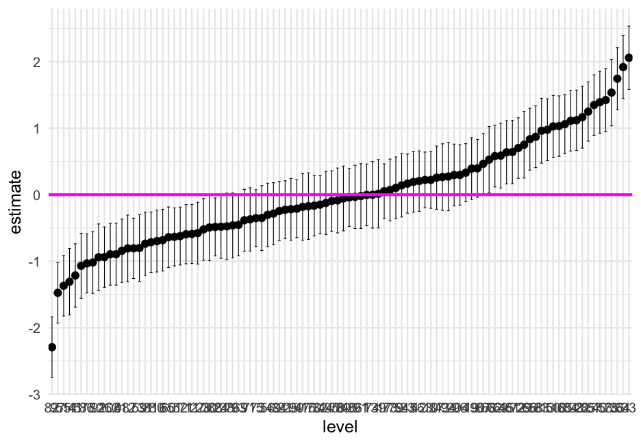Copy Code

Wrapping up coef plots

• Coefficient plots are generally fairly easy to produce, but often not the most informative

• Random effects plots are probs more informative than the fixed effects/variance components plots

• You can make either a lot more fancy, accessible, etc., and probably should if you're going to use it for publication.

Reminder

Our raw data looks like this

popularCopy Code

## # A tibble: 2,000 x 7
##    pupil class extrav sex    texp popular popteach
##    <dbl> <dbl>  <dbl> <chr> <dbl>   <dbl>    <dbl>
##  1     1     1      5 girl     24     6.3        6
##  2     2     1      7 boy      24     4.9        5
##  3     3     1      4 girl     24     5.3        6
##  4     4     1      3 girl     24     4.7        5
##  5     5     1      5 girl     24     6          6
##  6     6     1      4 boy      24     4.7        5
##  7     7     1      5 boy      24     5.9        5
##  8     8     1      4 boy      24     4.2        5
##  9     9     1      5 boy      24     5.2        5
## 10    10     1      5 boy      24     3.9        3
## # … with 1,990 more rowsCopy Code

Thinking back

to standard regression

let's say we fit a model like this

m <- lm(popular ~ 1 + sex, data = popular)Copy Code

Our estimated model is

$$\widehat{popular}=4.28+1.57\left({\mathrm{sex}}_{\mathrm{girl}}\right)$$

Making a prediction

What would our model on the prior slide predict for the first student?

pupil1 <- popular[1, ]
pupil1Copy Code

## # A tibble: 1 x 7
##   pupil class extrav sex    texp popular popteach
##   <dbl> <dbl>  <dbl> <chr> <dbl>   <dbl>    <dbl>
## 1     1     1      5 girl     24     6.3        6Copy Code

coef(m)[1] + # intercept
  coef(m)[2] * (pupil1$sex == "girl")Copy Code

## (Intercept) 
##    5.853314Copy Code

predict(m)[1]Copy Code

##        1 
## 5.853314Copy Code

What about this model?

If we use the predict function for m2, we get

predict(m2)[1]Copy Code

##        1 
## 5.732849Copy Code

How does the model come up with this prediction?

Use the next few minutes to see if you can write code to replicate it "by hand" as we did with the standard regression model

Thinking through the model

• We have classroom random effects for the intercept and slope

• This means the prediction for an individual is made up of:

  • Overall intercept +
  • Overall slope +
  • Classroom intercept offset (diff of classroom intercept from overall intercept) +
  • Classroom slope offset (diff of classroom slope from overall slope)

Do it!

First look back at the data

popular[1, ]Copy Code

## # A tibble: 1 x 7
##   pupil class extrav sex    texp popular popteach
##   <dbl> <dbl>  <dbl> <chr> <dbl>   <dbl>    <dbl>
## 1     1     1      5 girl     24     6.3        6Copy Code

Next extract the ran_vals for the coresponding class

m2_ranvals <- tidy(m2, effects = "ran_vals")
class1_ranvals <- m2_ranvals %>% 
  filter(group == "class" & level == 1)
class1_ranvalsCopy Code

## # A tibble: 2 x 6
##   effect   group level term           estimate std.error
##   <chr>    <chr> <chr> <chr>             <dbl>     <dbl>
## 1 ran_vals class 1     (Intercept)  0.02657986 0.2240683
## 2 ran_vals class 1     sexgirl     -0.04272575 0.1956483Copy Code

Make prediction

fixef(m2)Copy Code

## (Intercept)     sexgirl 
##    4.396820    1.352175Copy Code

fixef(m2)[1] + fixef(m2)[2]*(popular[1, ]$sex == "girl") +
  class1_ranvals$estimate[1] + class1_ranvals$estimate[2]Copy Code

## (Intercept) 
##    5.732849Copy Code

Confirm

predict(m2)[1]Copy Code

##        1 
## 5.732849Copy Code

Challenge

• Without using the predict() function, calculate the predicted score for a boy in classroom 10 from m2

class10_ranvals <- m2_ranvals %>% 
  filter(group == "class" & level == 10)
fixef(m2)[1] + class10_ranvals$estimate[1]Copy Code

## (Intercept) 
##    4.675822Copy Code

Confirm with predict()

test <- popular %>% 
  mutate(pred = predict(m2)) %>% 
  filter(class == 10 & sex == "boy") 
testCopy Code

## # A tibble: 12 x 8
##    pupil class extrav sex    texp popular popteach     pred
##    <dbl> <dbl>  <dbl> <chr> <dbl>   <dbl>    <dbl>    <dbl>
##  1     1    10      5 boy      21     5.4        5 4.675822
##  2     3    10      5 boy      21     3.4        3 4.675822
##  3     5    10      5 boy      21     5.1        7 4.675822
##  4     7    10      5 boy      21     5.4        4 4.675822
##  5     8    10      5 boy      21     4.9        4 4.675822
##  6    11    10      6 boy      21     4.4        6 4.675822
##  7    12    10      6 boy      21     4.9        5 4.675822
##  8    14    10      6 boy      21     4.8        3 4.675822
##  9    15    10      3 boy      21     3.6        3 4.675822
## 10    16    10      5 boy      21     5          6 4.675822
## 11    17    10      3 boy      21     5.5        5 4.675822
## 12    18    10      6 boy      21     5          4 4.675822Copy Code

More on the predict function

• Once you have the model parameters, you can predict for any values of those parameters

Let's fit a slightly more complicated model, using a different longitudinal file than what you used (or are using) in the homework

library(equatiomatic)
head(sim_longitudinal)Copy Code

## # A tibble: 6 x 8
## # Groups:   school [1]
##     sid school district group  treatment  prop_low  wave    score
##   <int>  <int>    <int> <chr>  <fct>         <dbl> <dbl>    <dbl>
## 1     1      1        1 medium 1         0.1428571     0 102.2686
## 2     1      1        1 medium 1         0.1428571     1 102.0135
## 3     1      1        1 medium 1         0.1428571     2 102.5216
## 4     1      1        1 medium 1         0.1428571     3 102.2792
## 5     1      1        1 medium 1         0.1428571     4 102.2834
## 6     1      1        1 medium 1         0.1428571     5 102.7963Copy Code

Model

You try first

• Fit a model with wave and treatment as predictors of students' score. Allow the intercept and the relation between wave and score to vary by student.

m <- lmer(score ~ wave + treatment + (wave|sid),
          data = sim_longitudinal)Copy Code

Plot predictions

Let's first just limit our data to the first three students.

first_three <- sim_longitudinal %>% 
  ungroup() %>%
  filter(sid %in% 1:3)Copy Code

Now try creating a new column in the data with the model predictions for these students. Specify newdata = first_three to only make the predictions for those cases.

first_three %>% 
  mutate(model_pred = predict(m, newdata = first_three))Copy Code

## # A tibble: 30 x 9
##      sid school district group  treatment  prop_low  wave    score model_pred
##    <int>  <int>    <int> <chr>  <fct>         <dbl> <dbl>    <dbl>      <dbl>
##  1     1      1        1 medium 1         0.1428571     0 102.2686   101.9955
##  2     1      1        1 medium 1         0.1428571     1 102.0135   102.1572
##  3     1      1        1 medium 1         0.1428571     2 102.5216   102.3189
##  4     1      1        1 medium 1         0.1428571     3 102.2792   102.4806
##  5     1      1        1 medium 1         0.1428571     4 102.2834   102.6423
##  6     1      1        1 medium 1         0.1428571     5 102.7963   102.8040
##  7     1      1        1 medium 1         0.1428571     6 103.0441   102.9657
##  8     1      1        1 medium 1         0.1428571     7 102.8868   103.1274
##  9     1      1        1 medium 1         0.1428571     8 103.9101   103.2891
## 10     1      1        1 medium 1         0.1428571     9 103.2392   103.4508
## # … with 20 more rowsCopy Code

Plot

Try creating a plot with a different facet for each sid showing the observed trend (relation between wave and score) as compared to the model prediction. Color the line by whether or not the student was in the treatment group or not.

first_three %>% 
  mutate(model_pred = predict(m, newdata = first_three)) %>% 
  ggplot(aes(wave, score, color = treatment)) +
  geom_point() +
  geom_line() +
  geom_line(aes(y = model_pred)) +
  facet_wrap(~sid)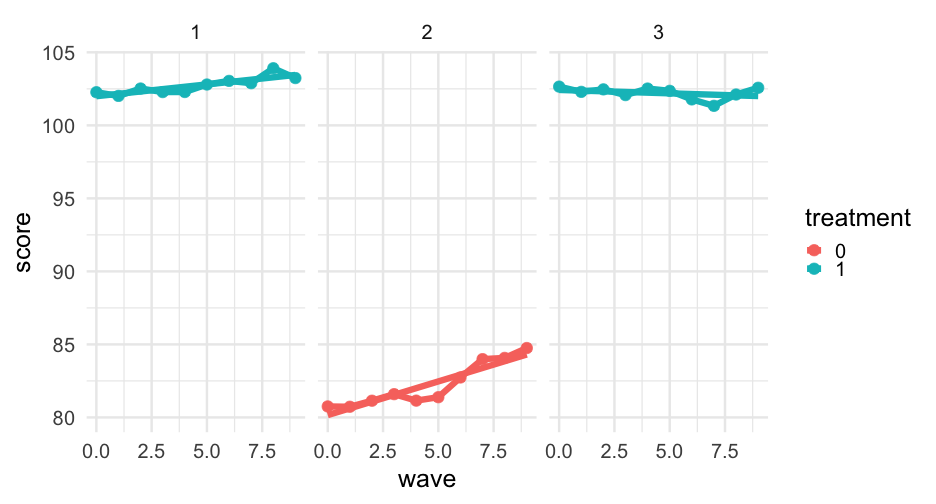Copy Code

Predictions outside our data

Student 2 has a considerably lower intercept. What would we predict the trend would look like if they had been in the treatment group?

Try to make this prediction on your own for all time points

stu2_trt <- data.frame(
  sid = 2,
  wave = 0:9,
  treatment = factor("1", levels = c(0, 1))
)
predict(m, newdata = stu2_trt)Copy Code

##        1        2        3        4        5        6        7        8 
## 78.61702 79.07803 79.53903 80.00004 80.46104 80.92205 81.38305 81.84406 
##        9       10 
## 82.30506 82.76607Copy Code

Compare

sim_longitudinal %>% 
  filter(sid == 2) %>% 
  mutate(model_pred = predict(m, newdata = .),
         trt_pred = predict(m, newdata = stu2_trt)) %>% 
  ggplot(aes(wave, score)) +
  geom_point() +
  geom_line() +
  geom_line(aes(y = model_pred)) +
  geom_line(aes(y = trt_pred),
            color = "firebrick") +
  annotate(
    "text", 
    x = 6, 
    y = 81, 
    hjust = 0, 
    color = "firebrick", 
    label = "Predicted slope if student\nwas in treatment group"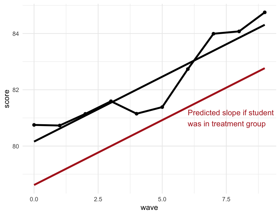
  )Copy Code

Wait... negative?

Yes...

arm::display(m)Copy Code

## lmer(formula = score ~ wave + treatment + (wave | sid), data = sim_longitudinal)
##             coef.est coef.se
## (Intercept) 97.95     1.38  
## wave         0.17     0.03  
## treatment1  -1.54     1.92  
## 
## Error terms:
##  Groups   Name        Std.Dev. Corr  
##  sid      (Intercept) 9.74           
##           wave        0.29     -0.16 
##  Residual             0.44           
## ---
## number of obs: 1000, groups: sid, 100
## AIC = 2407.7, DIC = 2393.1
## deviance = 2393.4Copy Code

Note - I'm just using an alternative function here to get it to fit on the slides easier

Other projections

We have a linear model. This means we can just extend the line to $\infty$ if we wanted to

🤪

newdata_stu2 <- data.frame(
  sid = 2,
  wave = rep(-500:500, 2),
  treatment = factor(rep(c(0, 1), each = length(-500:500)))
)Copy Code

newdata_stu2 %>% 
  mutate(pred = predict(m, newdata = newdata_stu2)) %>% 
  ggplot(aes(wave, pred)) +
  geom_line(aes(color = treatment))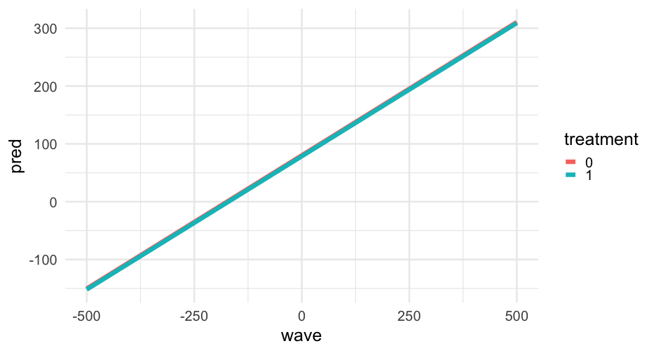Copy Code

What to predict?

Let's say we want to predict what time points 10, 11, and 12 would look like for the first three students.

First, create the prediction data frame

pred_frame <- data.frame(
  sid = rep(1:3, each = 13),
  wave = rep(0:12),
  treatment = factor(rep(c(1, 0, 1), each = 13))
)
head(pred_frame)Copy Code

##   sid wave treatment
## 1   1    0         1
## 2   1    1         1
## 3   1    2         1
## 4   1    3         1
## 5   1    4         1
## 6   1    5         1Copy Code

merTools

Next, load the {merTools} package

library(merTools)Copy Code

Create a prediction interval with predictInterval(), using simulation to obtain the prediction interval

m_pred_interval <- predictInterval(
  m, 
  newdata = pred_frame, 
  level = 0.95
)Copy Code

m_pred_intervalCopy Code

##          fit       upr       lwr
## 1  102.01207 104.72567  99.12815
## 2  102.21023 104.90541  99.27463
## 3  102.29546 105.12290  99.46212
## 4  102.51889 105.24485  99.46114
## 5  102.65108 105.36337  99.80513
## 6  102.76418 105.52242  99.74719
## 7  102.96957 105.60124  99.88279
## 8  103.12596 105.79933 100.20903
## 9  103.29646 105.97636 100.38468
## 10 103.45665 106.11203 100.42733
## 11 103.67235 106.41096 100.59995
## 12 103.79786 106.50498 100.71008
## 13 103.94205 106.78566 100.93741
## 14  80.09841  82.96316  77.35830
## 15  80.57764  83.33608  77.88836
## 16  80.95438  83.81905  78.29942
## 17  81.52330  84.29985  78.74763
## 18  82.00058  84.70749  79.31407
## 19  82.41634  85.17683  79.85975
## 20  82.90433  85.69380  80.15920
## 21  83.32670  86.17170  80.72806
## 22  83.74488  86.63404  81.06728
## 23  84.31655  87.24745  81.60025
## 24  84.71815  87.79115  82.10399
## 25  85.14727  88.28133  82.40308
## 26  85.65959  88.65188  82.85234
## 27 102.45376 105.27047  99.71076
## 28 102.38756 105.17645  99.56086
## 29 102.32892 105.19029  99.46407
## 30 102.32501 104.91057  99.37041
## 31 102.21161 104.91994  99.54185
## 32 102.20953 104.91597  99.29393
## 33 102.14807 104.84285  99.16836
## 34 102.02224 104.84638  99.18406
## 35 102.03473 104.67471  99.02696
## 36 101.97196 104.73033  99.07564
## 37 101.96588 104.69053  98.99436
## 38 101.84893 104.56803  98.71735
## 39 101.82603 104.67284  98.61854Copy Code

Binding data together

Let's add these predictions back to our prediction data frame, then plot them

bind_cols(pred_frame, m_pred_interval)Copy Code

##    sid wave treatment       fit       upr       lwr
## 1    1    0         1 102.01207 104.72567  99.12815
## 2    1    1         1 102.21023 104.90541  99.27463
## 3    1    2         1 102.29546 105.12290  99.46212
## 4    1    3         1 102.51889 105.24485  99.46114
## 5    1    4         1 102.65108 105.36337  99.80513
## 6    1    5         1 102.76418 105.52242  99.74719
## 7    1    6         1 102.96957 105.60124  99.88279
## 8    1    7         1 103.12596 105.79933 100.20903
## 9    1    8         1 103.29646 105.97636 100.38468
## 10   1    9         1 103.45665 106.11203 100.42733
## 11   1   10         1 103.67235 106.41096 100.59995
## 12   1   11         1 103.79786 106.50498 100.71008
## 13   1   12         1 103.94205 106.78566 100.93741
## 14   2    0         0  80.09841  82.96316  77.35830
## 15   2    1         0  80.57764  83.33608  77.88836
## 16   2    2         0  80.95438  83.81905  78.29942
## 17   2    3         0  81.52330  84.29985  78.74763
## 18   2    4         0  82.00058  84.70749  79.31407
## 19   2    5         0  82.41634  85.17683  79.85975
## 20   2    6         0  82.90433  85.69380  80.15920
## 21   2    7         0  83.32670  86.17170  80.72806
## 22   2    8         0  83.74488  86.63404  81.06728
## 23   2    9         0  84.31655  87.24745  81.60025
## 24   2   10         0  84.71815  87.79115  82.10399
## 25   2   11         0  85.14727  88.28133  82.40308
## 26   2   12         0  85.65959  88.65188  82.85234
## 27   3    0         1 102.45376 105.27047  99.71076
## 28   3    1         1 102.38756 105.17645  99.56086
## 29   3    2         1 102.32892 105.19029  99.46407
## 30   3    3         1 102.32501 104.91057  99.37041
## 31   3    4         1 102.21161 104.91994  99.54185
## 32   3    5         1 102.20953 104.91597  99.29393
## 33   3    6         1 102.14807 104.84285  99.16836
## 34   3    7         1 102.02224 104.84638  99.18406
## 35   3    8         1 102.03473 104.67471  99.02696
## 36   3    9         1 101.97196 104.73033  99.07564
## 37   3   10         1 101.96588 104.69053  98.99436
## 38   3   11         1 101.84893 104.56803  98.71735
## 39   3   12         1 101.82603 104.67284  98.61854Copy Code

Plot

bind_cols(pred_frame, m_pred_interval) %>% 
  ggplot(aes(wave, fit)) +
  geom_ribbon(aes(ymin = lwr, ymax = upr),
              alpha = 0.4) +
  geom_line(color = "magenta") +
  facet_wrap(~sid)Copy Code

How?

What's really going on here?

See here for a full description, but basically:

1. Creates a simulated (with n.sim samples) distribution for each model parameter
2. Computes a distribution of predictions
3. Returns the specifics of the prediction distribution, as requested (e.g., fit is the mean or median, and upr and lwr are the corresponding quaniteles for the uncertainty range)

Disclaimer

According to the {lme4} authors

There is no option for computing standard errors of predictions because it is difficult to define an efficient method that incorporates uncertainty in the variance parameters; we recommend lme4::bootMer() for this task.

The predictInterval() function is an approximation, while bootMer() is the "gold standard" (it just takes a long time)

Boostrapping

Write a function to compute the predictions for each bootstrap resample

pred_fun <- function(fit) {
  predict(fit, newdata = pred_frame)
}Copy Code

Notice we're using the same prediction data frame

Now create BS Estimates

Note this takes a few seconds, and for bigger models may take a long time

b <- bootMer(
  m, 
  nsim = 1000, 
  FUN = pred_fun,
  use.u = TRUE, 
  seed = 42
)Copy Code

The predictions are stored in a matrix t

dim(b$t)Copy Code

## [1] 1000   39Copy Code

Each row of the matrix is the prediction for the given bootstrap estimate

Lots of options

There are lots of things you could do with this now. I'll move it to a data frame first

bd <- as.data.frame(t(b$t)) %>% 
  mutate(sid = rep(1:3, each = 13),
         wave = rep(0:12, 3)) %>% 
  pivot_longer(
    starts_with("V"),
    names_to = "bootstrap_sample",
    names_prefix = "V",
    names_transform = list(bootstrap_sample = as.numeric),
    values_to = "score"
  ) %>% 
  arrange(sid, bootstrap_sample, wave)Copy Code

bdCopy Code

## # A tibble: 39,000 x 4
##      sid  wave bootstrap_sample    score
##    <int> <int>            <dbl>    <dbl>
##  1     1     0                1 102.1749
##  2     1     1                1 102.3497
##  3     1     2                1 102.5245
##  4     1     3                1 102.6992
##  5     1     4                1 102.8740
##  6     1     5                1 103.0488
##  7     1     6                1 103.2235
##  8     1     7                1 103.3983
##  9     1     8                1 103.5731
## 10     1     9                1 103.7478
## # … with 38,990 more rowsCopy Code

Plot

ggplot(bd, aes(wave, score)) +
  geom_line(aes(group = bootstrap_sample),
            size = 0.1,
            alpha = 0.5,
            color = "cornflowerblue") +
  facet_wrap(~sid)Copy Code

Prefer ribbons?

bd_ribbons <- bd %>% 
  group_by(sid, wave) %>% 
  summarize(quantile = quantile(score, c(0.025, 0.975)),
            group = c("lower", "upper")) %>% 
  pivot_wider(names_from = "group", values_from = "quantile")
bd_ribbonsCopy Code

## # A tibble: 39 x 4
## # Groups:   sid, wave [39]
##      sid  wave    lower    upper
##    <int> <int>    <dbl>    <dbl>
##  1     1     0 101.4553 102.4854
##  2     1     1 101.7114 102.5782
##  3     1     2 101.9408 102.6748
##  4     1     3 102.1633 102.7898
##  5     1     4 102.3576 102.9110
##  6     1     5 102.5236 103.0809
##  7     1     6 102.6428 103.2611
##  8     1     7 102.7468 103.4728
##  9     1     8 102.8555 103.6996
## 10     1     9 102.9428 103.9153
## # … with 29 more rowsCopy Code

Join with real data

bd_ribbons <- left_join(first_three, bd_ribbons) %>% 
  mutate(pred = predict(m, newdata = first_three))Copy Code

## Joining, by = c("sid", "wave")Copy Code

Plot again

ggplot(bd_ribbons, aes(wave, score)) +
  geom_ribbon(aes(ymin = lower, ymax = upper),
              alpha = 0.5) +
  geom_line(aes(y = pred), size = 1, color = "magenta") +
  geom_point() +
  facet_wrap(~sid)Copy Code

Important

There are different types of bootstrap resampling you can choose from

• Do you want to randomly sample from the random effects also? use.u = FALSE

• Do you want to assume the random effect estimates are true, and just sample the rest? use.u = TRUE

Honestly - this is a bit confusing to me, and the results from use.u = FALSE didn't make much sense to me. But see here and here for more information

Interactions

Let's create an interaction between treatment and wave

Conceptually: what would this mean?

Let's also add in a school-level random effect for the intercept

Interactions

Specified just like with lm(). Each of the below are equivalent

wave + treatment + wave:treatmentCopy Code

wave * treatmentCopy Code

where the latter just expands out to the former.

Adding additional levels

There are a few ways to do this:

• Assume your IDs are all unique
  • implicit nesting
• Don't worry and the IDs, and specify the nesting through the formula
  • Will result in equivalent estimates if the IDs are unique

See here for more examples

Implicit nesting

m1a <- lmer(score ~ wave*treatment + 
              (wave|sid) + (1|school),
            data = sim_longitudinal)
arm::display(m1a)Copy Code

## lmer(formula = score ~ wave * treatment + (wave | sid) + (1 | 
##     school), data = sim_longitudinal)
##                 coef.est coef.se
## (Intercept)     96.80     1.57  
## wave             0.40     0.03  
## treatment1       0.61     1.88  
## wave:treatment1 -0.45     0.04  
## 
## Error terms:
##  Groups   Name        Std.Dev. Corr  
##  sid      (Intercept) 9.16           
##           wave        0.19     -0.13 
##  school   (Intercept) 3.27           
##  Residual             0.44           
## ---
## number of obs: 1000, groups: sid, 100; school, 15
## AIC = 2330, DIC = 2301.2
## deviance = 2306.6Copy Code

Explicit nesting

m1b <- lmer(score ~ wave*treatment + 
              (wave|sid:school) + (1|school) ,
            data = sim_longitudinal)
arm::display(m1b)Copy Code

## lmer(formula = score ~ wave * treatment + (wave | sid:school) + 
##     (1 | school), data = sim_longitudinal)
##                 coef.est coef.se
## (Intercept)     96.80     1.57  
## wave             0.40     0.03  
## treatment1       0.61     1.88  
## wave:treatment1 -0.45     0.04  
## 
## Error terms:
##  Groups     Name        Std.Dev. Corr  
##  sid:school (Intercept) 9.16           
##             wave        0.19     -0.13 
##  school     (Intercept) 3.27           
##  Residual               0.44           
## ---
## number of obs: 1000, groups: sid:school, 100; school, 15
## AIC = 2330, DIC = 2301.2
## deviance = 2306.6Copy Code

Predictions "by hand"

This is now a three-level model. How does it differ from two-level models in terms of model predictions?

Let's make a prediction for the first student at the fourth time point:

sim_longitudinal[4, ]Copy Code

## # A tibble: 1 x 8
## # Groups:   school [1]
##     sid school district group  treatment  prop_low  wave    score
##   <int>  <int>    <int> <chr>  <fct>         <dbl> <dbl>    <dbl>
## 1     1      1        1 medium 1         0.1428571     3 102.2792Copy Code

The pieces

fixed <- fixef(m1a)
ranefs <- ranef(m1a)
fixedCopy Code

##     (Intercept)            wave      treatment1 wave:treatment1 
##      96.7973387       0.4010222       0.6080336      -0.4459053Copy Code

# Pull just the ranefs for sid 1 and school 1
sid_ranefs <- ranefs$sid[1, ] 
sid_ranefsCopy Code

##   (Intercept)      wave
## 1     1.85279 0.1936603Copy Code

sch_ranefs <- ranefs$school[1, ]
sch_ranefsCopy Code

## [1] 2.795928Copy Code

Putting it together

(fixed[1] + sid_ranefs[1] + sch_ranefs) + # intercept
((fixed[2] + sid_ranefs[2]) * 3) + # fourth timepoint
(fixed[3] * 1) + # treatment effect
(fixed[4] * 3)  # treatment by wave effectCopy Code

##   (Intercept)
## 1    102.5004Copy Code

Confirm

predict(m1a, newdata = sim_longitudinal[4, ])Copy Code

##        1 
## 102.5004Copy Code

Predictions

Let's randomly sample 5 students in the first four school and display the model predictions for those students.

There are many ways to create the sample, here's one:

samp <- sim_longitudinal %>% 
  filter(school %in% 1:4) %>% 
  group_by(school, sid) %>% 
  nest()
sampCopy Code

## # A tibble: 28 x 3
## # Groups:   sid, school [28]
##      sid school data             
##    <int>  <int> <list>           
##  1     1      1 <tibble [10 × 6]>
##  2    33      3 <tibble [10 × 6]>
##  3    34      4 <tibble [10 × 6]>
##  4    46      1 <tibble [10 × 6]>
##  5    61      1 <tibble [10 × 6]>
##  6    77      2 <tibble [10 × 6]>
##  7    78      3 <tibble [10 × 6]>
##  8    91      1 <tibble [10 × 6]>
##  9    93      3 <tibble [10 × 6]>
## 10     2      2 <tibble [10 × 6]>
## # … with 18 more rowsCopy Code

Select 5 rows for each school

set.seed(42)
samp %>% 
  group_by(school) %>% 
  sample_n(5)Copy Code

## # A tibble: 20 x 3
## # Groups:   school [4]
##      sid school data             
##    <int>  <int> <list>           
##  1     1      1 <tibble [10 × 6]>
##  2    76      1 <tibble [10 × 6]>
##  3    31      1 <tibble [10 × 6]>
##  4    16      1 <tibble [10 × 6]>
##  5    46      1 <tibble [10 × 6]>
##  6    62      2 <tibble [10 × 6]>
##  7     2      2 <tibble [10 × 6]>
##  8    92      2 <tibble [10 × 6]>
##  9    77      2 <tibble [10 × 6]>
## 10    47      2 <tibble [10 × 6]>
## 11    63      3 <tibble [10 × 6]>
## 12    18      3 <tibble [10 × 6]>
## 13    33      3 <tibble [10 × 6]>
## 14    48      3 <tibble [10 × 6]>
## 15    78      3 <tibble [10 × 6]>
## 16    19      4 <tibble [10 × 6]>
## 17    49      4 <tibble [10 × 6]>
## 18     4      4 <tibble [10 × 6]>
## 19    79      4 <tibble [10 × 6]>
## 20    94      4 <tibble [10 × 6]>Copy Code

unnest()

set.seed(42)
samp <- samp %>% 
  group_by(school) %>% 
  sample_n(5) %>% 
  unnest(data) %>% 
  ungroup()
sampCopy Code

## # A tibble: 200 x 8
##      sid school district group  treatment  prop_low  wave    score
##    <int>  <int>    <int> <chr>  <fct>         <dbl> <dbl>    <dbl>
##  1     1      1        1 medium 1         0.1428571     0 102.2686
##  2     1      1        1 medium 1         0.1428571     1 102.0135
##  3     1      1        1 medium 1         0.1428571     2 102.5216
##  4     1      1        1 medium 1         0.1428571     3 102.2792
##  5     1      1        1 medium 1         0.1428571     4 102.2834
##  6     1      1        1 medium 1         0.1428571     5 102.7963
##  7     1      1        1 medium 1         0.1428571     6 103.0441
##  8     1      1        1 medium 1         0.1428571     7 102.8868
##  9     1      1        1 medium 1         0.1428571     8 103.9101
## 10     1      1        1 medium 1         0.1428571     9 103.2392
## # … with 190 more rowsCopy Code

Make prediction

samp %>% 
  mutate(pred = predict(m1a, newdata = samp))Copy Code

## # A tibble: 200 x 9
##      sid school district group  treatment  prop_low  wave    score     pred
##    <int>  <int>    <int> <chr>  <fct>         <dbl> <dbl>    <dbl>    <dbl>
##  1     1      1        1 medium 1         0.1428571     0 102.2686 102.0541
##  2     1      1        1 medium 1         0.1428571     1 102.0135 102.2029
##  3     1      1        1 medium 1         0.1428571     2 102.5216 102.3516
##  4     1      1        1 medium 1         0.1428571     3 102.2792 102.5004
##  5     1      1        1 medium 1         0.1428571     4 102.2834 102.6492
##  6     1      1        1 medium 1         0.1428571     5 102.7963 102.7980
##  7     1      1        1 medium 1         0.1428571     6 103.0441 102.9468
##  8     1      1        1 medium 1         0.1428571     7 102.8868 103.0955
##  9     1      1        1 medium 1         0.1428571     8 103.9101 103.2443
## 10     1      1        1 medium 1         0.1428571     9 103.2392 103.3931
## # … with 190 more rowsCopy Code

Plot

samp %>% 
  mutate(pred = predict(m1a, newdata = samp)) %>% 
  ggplot(aes(wave, pred, group = sid)) +
  geom_line() +
  facet_wrap(~school)Copy Code

Marginal effect

A marginal effect shows the relation between one variable in the model and the outcome, while averaging over the other predictors in the model

Let's start by making the models slightly more complicated

m2 <- lmer(score ~ wave*treatment + group + prop_low +
              (wave|sid) + (1|school) ,
            data = sim_longitudinal)Copy Code

arm::display(m2, detail = TRUE)Copy Code

## lmer(formula = score ~ wave * treatment + group + prop_low + 
##     (wave | sid) + (1 | school), data = sim_longitudinal)
##                 coef.est coef.se t value
## (Intercept)      97.62     4.70   20.78 
## wave              0.40     0.03   14.38 
## treatment1        0.82     1.91    0.43 
## grouplow         -4.83     4.00   -1.21 
## groupmedium      -3.61     3.75   -0.96 
## prop_low          9.34    10.21    0.91 
## wave:treatment1  -0.45     0.04  -11.42 
## 
## Error terms:
##  Groups   Name        Std.Dev. Corr  
##  sid      (Intercept) 9.18           
##           wave        0.19     -0.13 
##  school   (Intercept) 3.41           
##  Residual             0.44           
## ---
## number of obs: 1000, groups: sid, 100; school, 15
## AIC = 2319.8, DIC = 2313.2
## deviance = 2304.5Copy Code

Marginal effect

Let's look at the relation between wave and score by treatment, holding the other values constant.

First, build a prediction data frame. We'll make population-level prediction - i.e., ignoring the random effects.

marginal_frame1 <- data.frame(
  wave = rep(0:9, 2),
  treatment = as.factor(rep(c(0, 1), each = 10)),
  group = factor("high", levels = c("low", "medium", "high")),
  prop_low = mean(sim_longitudinal$prop_low, na.rm = TRUE),
  sid = -999,
  school = -999
)Copy Code

The length of each of these variables can sometimes get a little tricky

marginal_frame1Copy Code

##    wave treatment group prop_low  sid school
## 1     0         0  high      0.3 -999   -999
## 2     1         0  high      0.3 -999   -999
## 3     2         0  high      0.3 -999   -999
## 4     3         0  high      0.3 -999   -999
## 5     4         0  high      0.3 -999   -999
## 6     5         0  high      0.3 -999   -999
## 7     6         0  high      0.3 -999   -999
## 8     7         0  high      0.3 -999   -999
## 9     8         0  high      0.3 -999   -999
## 10    9         0  high      0.3 -999   -999
## 11    0         1  high      0.3 -999   -999
## 12    1         1  high      0.3 -999   -999
## 13    2         1  high      0.3 -999   -999
## 14    3         1  high      0.3 -999   -999
## 15    4         1  high      0.3 -999   -999
## 16    5         1  high      0.3 -999   -999
## 17    6         1  high      0.3 -999   -999
## 18    7         1  high      0.3 -999   -999
## 19    8         1  high      0.3 -999   -999
## 20    9         1  high      0.3 -999   -999Copy Code

Make predictions!

Note that we have to specify to allow new levels

marginal_frame1 <- marginal_frame1 %>% 
  mutate(pred = predict(m2, 
                        newdata = marginal_frame1, 
                        allow.new.levels = TRUE))
marginal_frame1Copy Code

##    wave treatment group prop_low  sid school     pred
## 1     0         0  high      0.3 -999   -999 100.4186
## 2     1         0  high      0.3 -999   -999 100.8196
## 3     2         0  high      0.3 -999   -999 101.2207
## 4     3         0  high      0.3 -999   -999 101.6217
## 5     4         0  high      0.3 -999   -999 102.0227
## 6     5         0  high      0.3 -999   -999 102.4237
## 7     6         0  high      0.3 -999   -999 102.8248
## 8     7         0  high      0.3 -999   -999 103.2258
## 9     8         0  high      0.3 -999   -999 103.6268
## 10    9         0  high      0.3 -999   -999 104.0278
## 11    0         1  high      0.3 -999   -999 101.2433
## 12    1         1  high      0.3 -999   -999 101.1984
## 13    2         1  high      0.3 -999   -999 101.1536
## 14    3         1  high      0.3 -999   -999 101.1087
## 15    4         1  high      0.3 -999   -999 101.0638
## 16    5         1  high      0.3 -999   -999 101.0189
## 17    6         1  high      0.3 -999   -999 100.9740
## 18    7         1  high      0.3 -999   -999 100.9291
## 19    8         1  high      0.3 -999   -999 100.8843
## 20    9         1  high      0.3 -999   -999 100.8394Copy Code

Plot it

ggplot(marginal_frame1, aes(wave, pred, color = treatment)) +
  geom_line()Copy Code

Why do this?

As the model gets more complicated, it can be increasingly difficult to understand the fixed effects.

Plotting the marginal effects regularly helps (e.g., for interactions and non-linear terms)

Try again

This time, let's look at the same thing, but for all groups, still holding prop_low constant.

marginal_frame2 <- data.frame(
  wave = rep(0:9, 2*3),
  treatment = as.factor(rep(c(0, 1), each = 10*3)),
  group = factor(
    rep(
      rep(c("low", "medium", "high"), each = 10),
      2
    )
  ),
  prop_low = mean(sim_longitudinal$prop_low, na.rm = TRUE),
  sid = -999,
  school = -999
)Copy Code

Predict & plot

marginal_frame2 %>% 
  mutate(
    pred = predict(m2, 
                   newdata = marginal_frame2, 
                   allow.new.levels = TRUE)
  ) %>% 
  ggplot(aes(wave, pred, color = treatment)) +
  geom_line() +
  facet_wrap(~group)Copy Code

Automated method

We can build this up on our own with new data frames

library(ggeffects)
ggpredict(m2, "wave")Copy Code

## # Predicted values of score
## # x = wave
## 
## x | Predicted |          95% CI
## -------------------------------
## 0 |    100.42 | [93.05, 107.78]
## 1 |    100.82 | [93.46, 108.18]
## 2 |    101.22 | [93.86, 108.58]
## 3 |    101.62 | [94.26, 108.98]
## 5 |    102.42 | [95.07, 109.78]
## 6 |    102.82 | [95.47, 110.18]
## 7 |    103.23 | [95.87, 110.58]
## 9 |    104.03 | [96.67, 111.39]
## 
## Adjusted for:
## * treatment =    0
## *     group = high
## *  prop_low = 0.30
## *       sid = 0 (population-level)
## *    school = 0 (population-level)Copy Code

Even automated plotting!

ggpredict(m2, c("wave", "treatment")) %>% 
  plot()Copy Code

Individual observation

We can get these prediction intervals for specific levels also

ggpredict(m2, "wave", condition = c(sid = 1, school = 1))Copy Code

## # Predicted values of score
## # x = wave
## 
## x | Predicted |          95% CI
## -------------------------------
## 0 |    100.42 | [93.05, 107.78]
## 1 |    100.82 | [93.46, 108.18]
## 2 |    101.22 | [93.86, 108.58]
## 3 |    101.62 | [94.26, 108.98]
## 5 |    102.42 | [95.07, 109.78]
## 6 |    102.82 | [95.47, 110.18]
## 7 |    103.23 | [95.87, 110.58]
## 9 |    104.03 | [96.67, 111.39]
## 
## Adjusted for:
## * treatment =    0
## *     group = high
## *  prop_low = 0.30Copy Code

All categorical groups

Note - things aren't perfect here, but it's still helpful.

ggpredict(m2, c("wave", "treatment", "group"), 
          condition = c(sid = 1, school = 1)) %>% 
  plot()Copy Code